Basic Usage
Everything you need to know about using permittivitycalc: github.com/boivinalex/permittivitycalc.
Housekeeping
For information on what permittivitycalc is for and how to install it see the README on github.
Issues with or questions about this tutorial or permittivitycalc itself can be reported on the issue tracker.
Introduction
permittivitycalc works by storing input S-parameter data and associated processed data in a Python Class called AirlineData. When data is input into permittivitycalc, a new instance of the AirlineData Class is created.
The AirlineData Class contains several data attributes and methods.
Data attributes store the raw S-parameter data, processed (complex permittivity, permeability) data, as well as variables. Some variables are mandatory such as the length of the transmission line (L), and some are optional such as the bulk density of the sample measured (bulk_density).
Methods are functions which either automatically process the input data, can be called to process data if an argument is given to the AirlineData Class Instance, or must be called manually.
In addition to the class methods, permittivitycalc also has additional helper functions which are used to input data (either manually or via file dialog), to plot both the permittivity data and the raw S-parameter data, and to plot multiple permittivity datasets together.
This tutorial is intended to demonstrate the features of permittivitycalc starting with basic usage and moving on to more advanced, custom, or minor features.
Tutorial
Basic Usage
0.9.14
3.0rc2
permittivitycalc contains two example datasets:
Rexolite
The maximum precentage difference between forward (S11/S21) and reverse (S22/S12) calculated permittivity is:
ε′: 0.35% ε′′: 277.82% tanδ: 277.81%
The median precentage difference between forward (S11/S21) and reverse (S22/S12) calculated permittivity is:
ε′: 0.02% ε′′: 18.24% tanδ: 18.22%


Serpentine
The maximum precentage difference between forward (S11/S21) and reverse (S22/S12) calculated permittivity is:
ε′: 1.20% ε′′: 129.94% tanδ: 130.00%
The median precentage difference between forward (S11/S21) and reverse (S22/S12) calculated permittivity is:
ε′: 0.10% ε′′: 5.69% tanδ: 5.60%
Each dataset is stored as an individual AirlineData instance. We can quickly get information about individual AirlineData instances like so:
Serpentine measured in VAL (L = 14.989) with a bulk density of 1.6 g/cm^3 from file:
/anaconda/envs/permittivitycalc/lib/python3.7/site-packages/permittivitycalc-0.6.0-py3.7.egg/permittivitycalc/data/serpentine_dry.txt
Similarly, we can get a Python readable expression which can be used to re-create the instance like so:
pc.AirlineData(*pc.get_METAS_data(airline='VAL',file_path='/anaconda/envs/permittivitycalc/lib/python3.7/site-packages/permittivitycalc-0.6.0-py3.7.egg/permittivitycalc/data/serpentine_dry.txt'),bulk_density=1.6,temperature=None,name='Serpentine',date=None,corr=False,solid_dielec=None,solid_losstan=None,particle_diameter=None,particle_density=None,nrw=False,normalize_density=False,norm_eqn='LI',shorted=False,freq_cutoff=100000000.0)
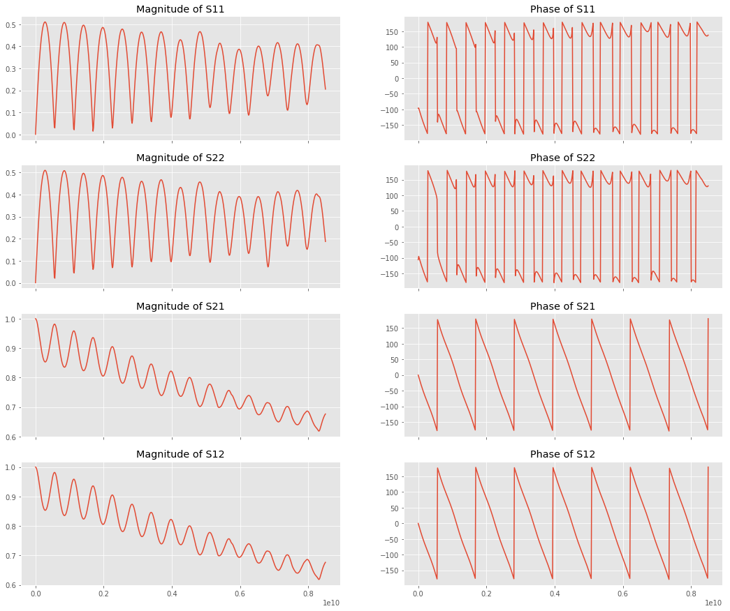
The S-parameters in the instance can be plotted like so:
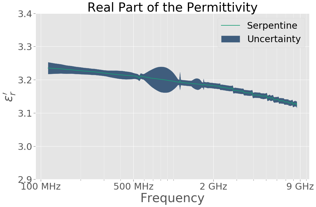
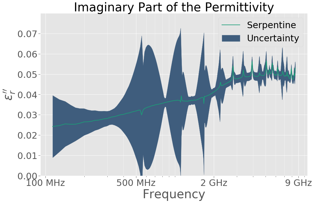
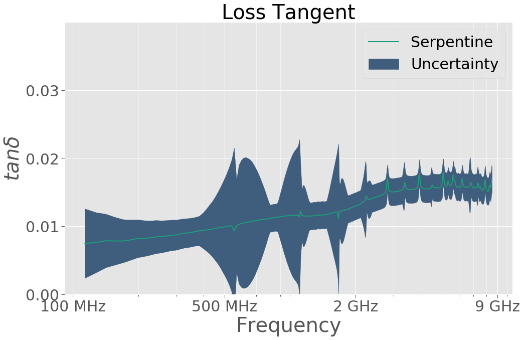
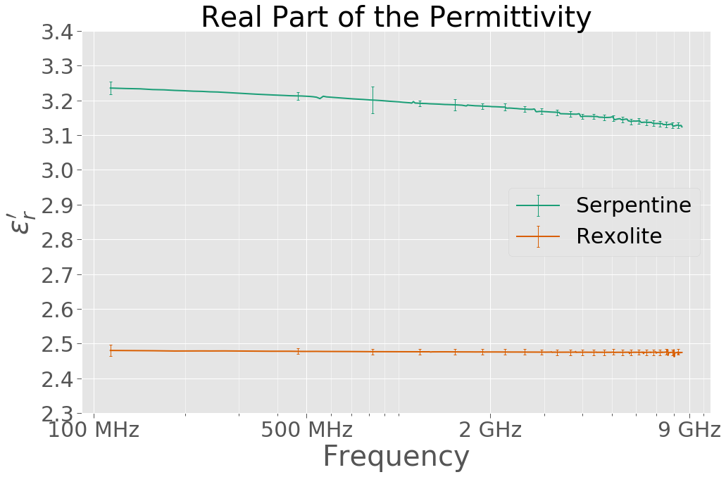
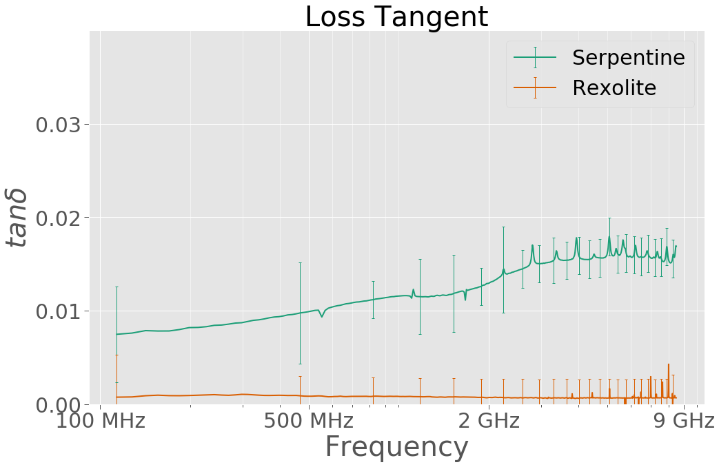
The calculated real part of the permittivity, imaginary part of the permittivity, and loss tangent can be plotted like so:
Two or more AirlineData instances can be compared to one another using the perm_compare function.
perm_compare requires a list of AirlineData instances to run. When more than one data set is being plotted, errorbars are shown every 25 points.
Basic File Input
permittivitycalc expects a tab delimited .txt file produced by saving the data table created in VNA Tools II. permittivitycalc will automatically determine whether the file contains uncertainties or not and propagate them automatically if they are present.
Note: File input is done via the helper function ``get_METAS_data`` and file in unpacked into in components by the ``_unpack`` method in AirlineData. If you want to input a file not produced in VNA Tools II, you will need to edit ``get_METAS_data`` and ``_unpack``.
The run_default function is the simplest way to input a file into
permittivitycalc. run_default needs an airline_name to run (Default:
'VAL'). The default corresponds to the GR900-LZ15 transmission line.
Running run_default will produce a File Dialog Prompt using tkinter.
instance_name = pc.run_default()
To use a different airline definition, simply set the airline_name.
Currently, the options are ‘VAL’, ‘PAL’, ‘GAL’, ‘7’, or ‘custom’. Using
‘custom’ will prompt you to input an airline length L in cm.
instance_name = pc.run_default(airline_name='custom')
Note: To create your own airline length definitions, edit the helper functions ``get_METAS_data`` and ``_get_file``
To open multiple files at once, the function multiple_meas can be
used.
list_of_instances = pc.multiple_meas()
multiple_meas will ask you which airline you are using. The name
must be given as a string. Once the airline_name is given a file
dialog will open. Selecting any .txt file in a folder will open all
other .txt files in that folder. All measurements must have been made in
the same airline.
The airline name can also be supplied directly:
list_of_instances = pc.multiple_meas(airline_name='custom')
multple_meas returns a list of AirlineData instances and plots all
input data together using perm_compare. Individual instances can be
accessed with indexing.
Example:
individual_instance = list_of_instances[0]
Saving Plots
Permittivity plots can be saved to the /Figues/ folder (folder will be
automatically created if it does not exist) by using the publish
argument. This feature does not currently exist for the S-parameter
plots.
Note: Currently, plots are saved as 300 dpi .eps files. These settings can be changed by editing the ``make_plot`` function in ``permittivity_plot.py``.
Example:
rexolite_example.draw_plots(publish=True)
Plots of multiple measurements can also be saved as long as a name is provided for the plots:
pc.perm_compare(multi_examples,name='save_name',publish=True)
Bulk Density Corrections
To correct powder measurements for bulk destiny, the bulk_density in
g/cm3 must be provided, normalize_density must be set to True
and, norm_eqn must be set to a valid string representing an equation
(Default: 'LI').
Currently, two equations are available for density normalization: - The
Lichtenecker equation ('LI') - Landau-Lifshitz-Looyenga equation
('LLL')
For information on how to use these equations see (Hickson, 2017)
Example:
instance_name = pc.run_default(bulk_density=1.8,normalize_density=True,norm_eqn='LLL')
Nicholson-Rross-Weir (NRW) Algorithm
By default, permittivity-plot uses the New Non-Iterative Method to
calculate the complex permittivity from S-parameters (Boughriet,
1997) which assumes \(\mu\) =
1 (non-magnetic). To use the NRW algorithm instead (Nicolson & Ross,
1970;Weir,
1974), nrw must be set
to True.
instance_name = pc.run_default(nrw=True)
Accessing The Data
When no uncertainties are provided in the input file, data in the AirlineData instance are stored as numpy arrays and can easily be accessed.
When uncertainties are provided, data are stored as
unumpy.uarray
objects where each value in the uarray has an uncertainty associated
with it.
For example, the computed permittivity arrays are stored as
avg_dielec, avg_lossfac, and avg_losstan.
Creating a copy of a data array simply requires accessing the relevant data attribute. For example:
For data when uncertainties, the nominal values can be extracted with
unp.nominal_values() and the uncertainties can be extracted with
unp.std_devs().